Models
Model types
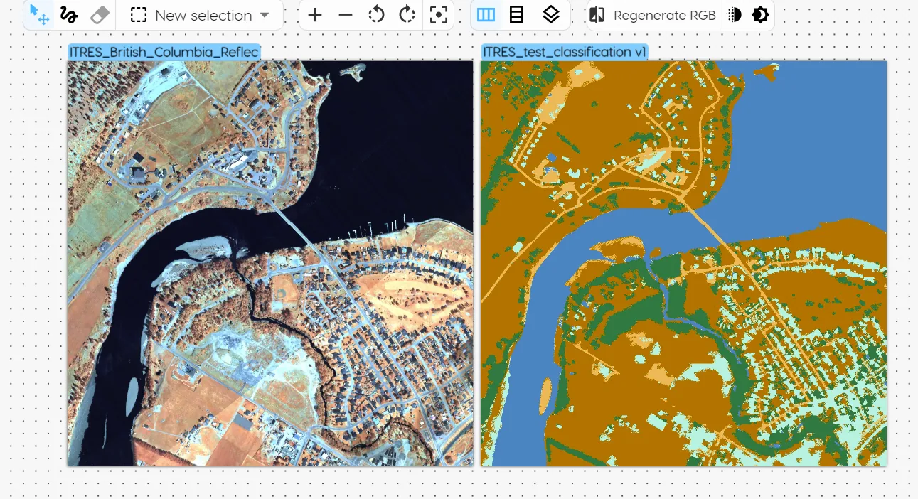
Classification
The classification model shows each labeled class as a separate color per pixel. Each selection in the training data should consist only of the spectral bands that correspond to the pure classes. The model then predicts which class a pixel belongs to.
- Use case: Classify one or more materials / surfaces in an image.
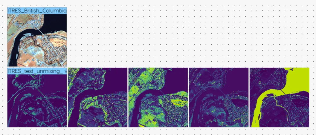
Unmixing
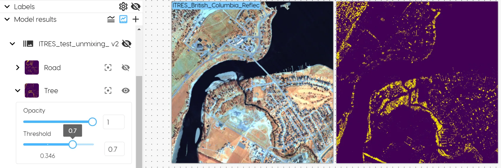
The unmixing model shows results for each endmember in a separate heatmap. The yellow depicts the abundance of the respective material (endmember), so the brighter the yellow, the greater the abundance of that material per pixel.
To filter out noise, you can toggle on "Confidence thresholds" in the toolbar. Confidence thresholds are set individually for each endmember, and tell the model the minimum percentage of a target endmember per pixel to visually depict.
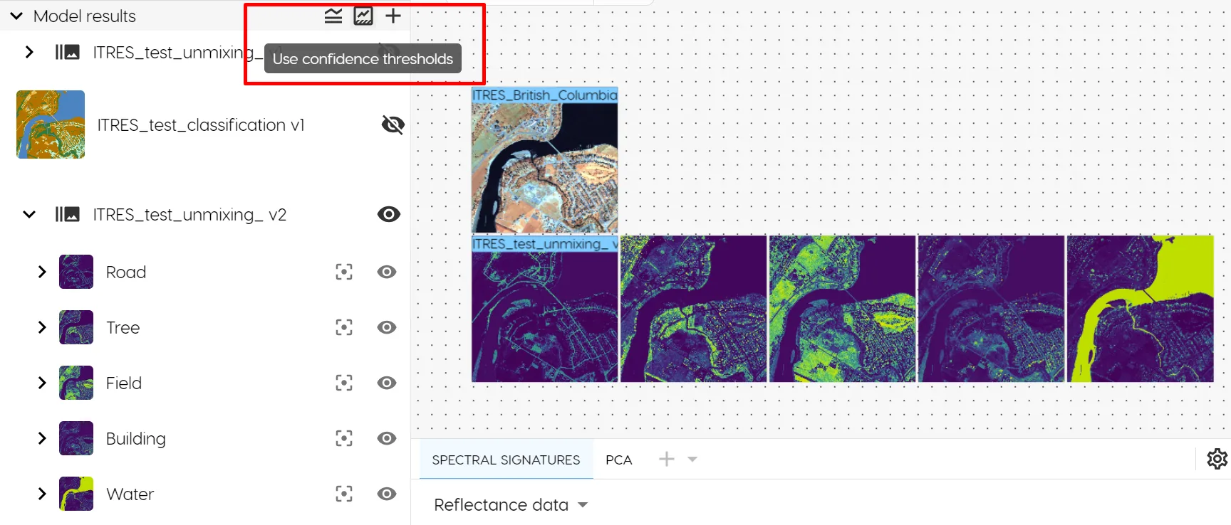
For example, a confidence threshold of 0 means that the model will identify any pixel where even the faintest detection of a spectral signature of your endmembers was detected. A confidence threshold of 1 means that the model will only identify pixels for which the composition consists exclusively (100%) of the spectral signature of your endmembers.
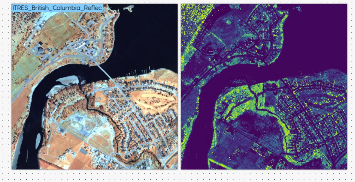
Depending on the endmembers you are looking to identify, you may adjust the confidence threshold per unmixing result image. Below is an example of fine tuning our model for tree identification using confidence treshholds.
- Use case: Provide images in the form of heatmaps of abundance for each endmember (i.e. one image per endmember). This can be used to understand if there are contaminants within a material, or if there are multiple materials present within a given pixel.
Target detection
This model identifies a specific class in an image. This is ideal for cases where a user wants to identify only one class with a high degree of confidence in an image. To train a target detection model, you will need a target class, as well as one or more non-targets. The non-targets can be any class in the image other than the target class.
Regression
This model predicts a continuous value for each pixel in an image. This is ideal for cases where a user wants to predict a continuous value for each pixel in an image, such as a reflectance value, or a chlorophyll content.
- Use case: Predict a continuous value for each pixel in an image.
Model training
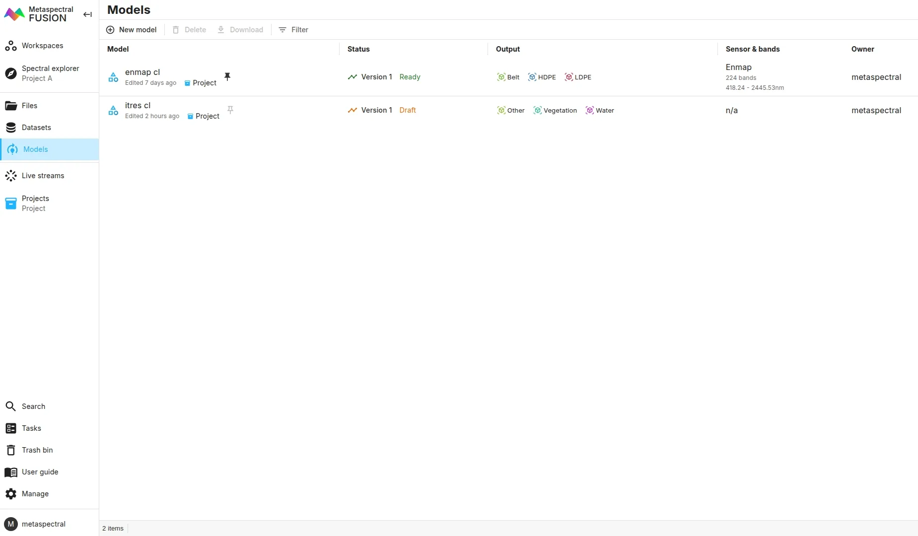
Go to the Models page and click New model.
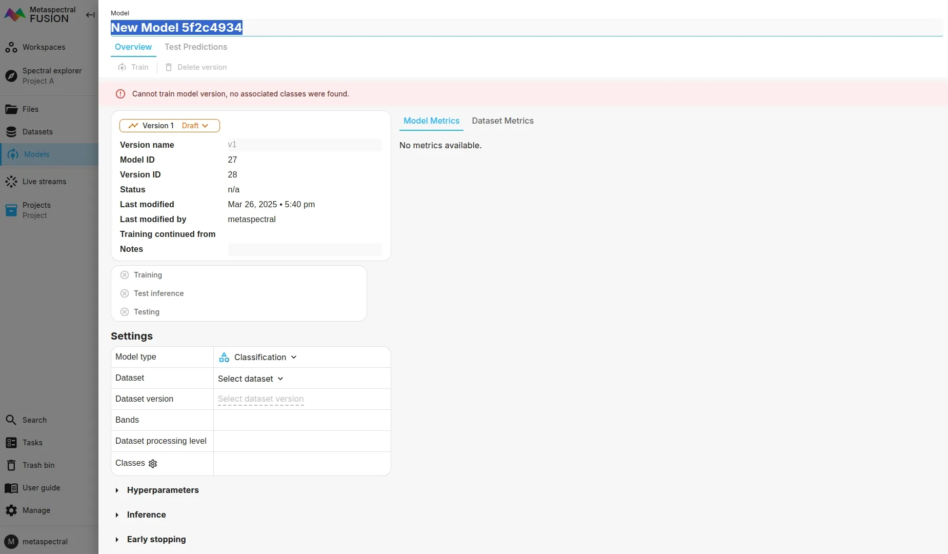
Select the model type, the dataset and version, and the other fields will automatically fill. The advanced deep learning settings are preset by default - you do not need to modify these unless you have experience with deep learning models and are looking to customize your model.
Click the Train button to train the model. If your dataset has test data, a test and inference run will be automatically performed.
Interpreting the results
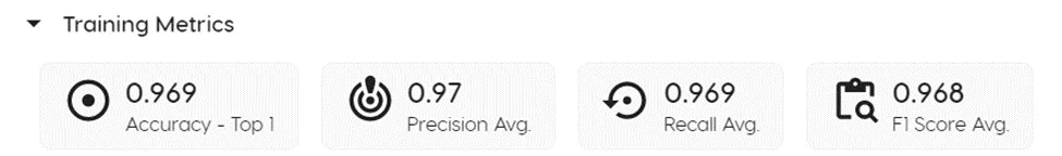
The first row of results, under the "Training Metrics" section measure the performance of the model training process.
Metrics
Accuracy
How well a model correctly classified instances out of the total instances it has evaluated. It is calculated as the ratio of correctly classified instances (both true positives and true negatives) to the total number of instances. A high accuracy (1 being 100%) means the model is good at identifying both positive and negative cases correctly. However, accuracy alone may not be a sufficient metric to evaluate model performance, especially when there is a class imbalance in the data. For instance, if 95% of the samples belong to class A, and the model always predicts class A, then the accuracy will be 95%, but the model is not really learning anything useful.
Precision
A measure of how well a model correctly identifies positive instances among those that it has predicted as positive. In other words, it tells you what proportion of the instances the model has labeled as positive are actually positive. A high precision means the model is good at avoiding false positives (incorrectly labeling negative instances as positive). High precision is particularly important in applications where false positives are costly, such as medical diagnoses or fraud detection.
Recall
Recall measures the ability of a classification model to identify all relevant instances (i.e., true positives) in the dataset, regardless of whether they are predicted as positive or negative by the model. In other words, recall measures the completeness of the model's predictions for the target class. A high recall means that the model can identify most or all of the relevant instances in the dataset, while a low recall means that the model misses many of the relevant instances.
F1 Score
The F1 score is a measure of the balance between precision and recall. It provides a way to evaluate the model's performance when both precision and recall are important. The F1 score ranges from 0 to 1, with higher values indicating better model performance.
Loss
The loss function measures the difference between the predicted values and the actual values. It is a measure of how well the model is able to fit the data. The loss function ranges from 0 to 1, with lower values indicating better model performance.
Error
The error function measures the difference between the predicted values and the actual values. It is a measure of how well the model is able to fit the data. The error function ranges from 0 to 1, with lower values indicating better model performance.
GradCAM
GradCAM is a method for visualizing the regions of an image that are important for the model's predictions. It is a post-hoc explanation method that can be used to understand the model's predictions.
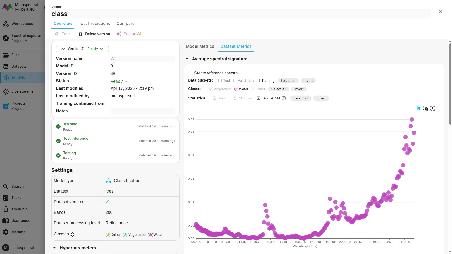
To view the GradCAM in Clarity, click on Dataset metrics after training your model, and then make sure Grad-CAM is enabled.
The busier the plot, the more important the region is for the model's predictions. You can also hover over the bands to see the corresponding values.
Unmixing models
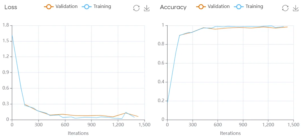
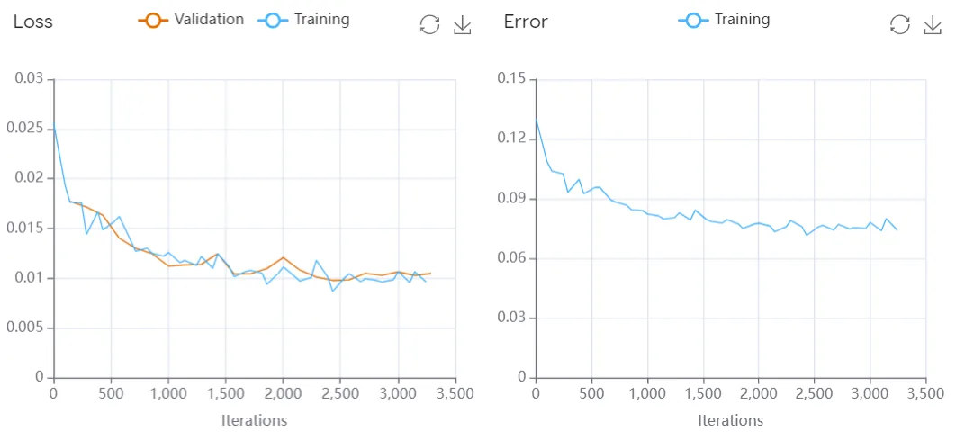
Loss function (classification and unmixing) - Evaluates the model's ability to generalize to new data by measuring how well the model makes predictions on the training data. It plots the loss function values over time during training (i.e., iterations). If the model is overfitting (i.e., performing well on the training data but poorly on the validation data), the loss on the training data will decrease over time while the loss on the validation data will increase. This results in a widening gap between the training and validation loss curves.
Accuracy function (classification) - Similar to the loss function, the accuracy graph tracks the training performance over time with a training and validation curve. However in this case, the graph shows the proportion of correct classifications made by the model over time, looking at how well the model is able to classify the targets it is trained on.
Error function: Shows how the error of a model changes over time. Error is a measure of how much the model's predictions differ from the actual values. In general, we want the error to decrease as the model learns more about the data.
Normalized confusion matrix
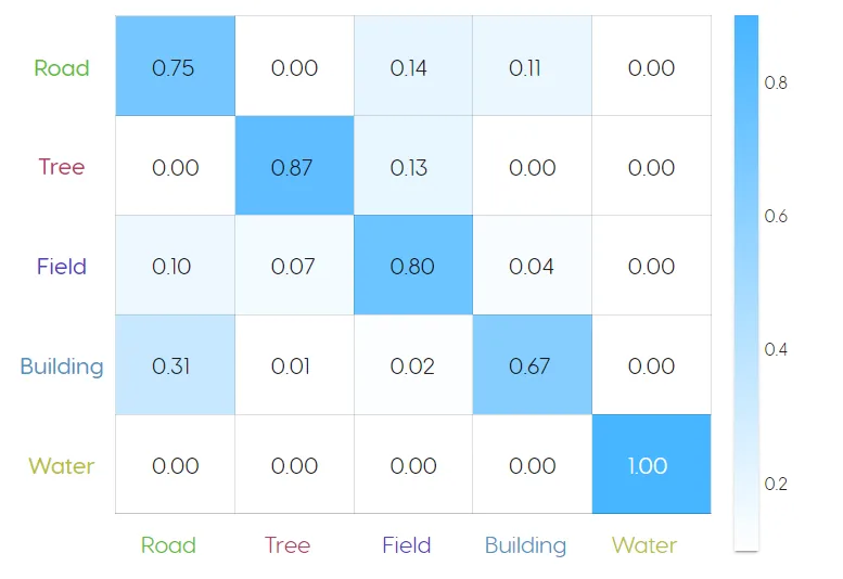
This shows what percentage of the model's classifications were correct for each class (1 = 100%). If a model is making incorrect classifications (i.e true / false positive, true / false negative), a non-0 value will appear in the upper right and lower left cells of the matrix.
**Evaluating performance: **
- The above unmixing model identified water with 100% accuracy, but only identified buildings with 67% accuracy, mistaking them for roads 31% of the time. This is likely due to the fact that some buildings have asphalt roofs, which is the same material as the roads.
- The performance can be improved by selecting more building and road examples for the training data, to allow the model to more effectively distinguish between the two spectral signatures.
- High accuracy doesn't necessary mean that the model performed well, as this can be a signal of overfitting. That is why it is important to evaluate model performance using the metrics discussed above, as well as visually audit its performance on new images that the model was not trained on.
Adjusting and improving the model
In the domain of statistical learning models, the first iteration of models created is rarely the best. Rather, the models can be significantly improved with adjustments after each iteration of testing. The adjustments made to the model will depend on your requirements for accuracy / precision / recall.
Versioning
Clarity supports iteration through the "Version" button available in both the Dataset and Model tabs.
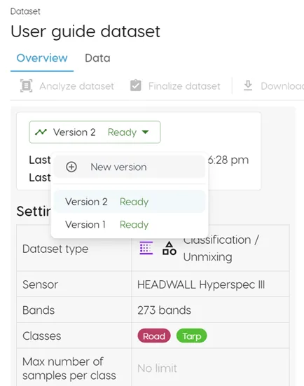
Click on the "Version" button, then "New version" to create a new iteration of either your dataset or associated model. You may want to do this if you decide to add additional selections or classes to your dataset, or train a model with different parameters. You can see each version as a toggleable layer in Spectral Explorer, making it easy to compare and contrast different versions of your dataset and model.
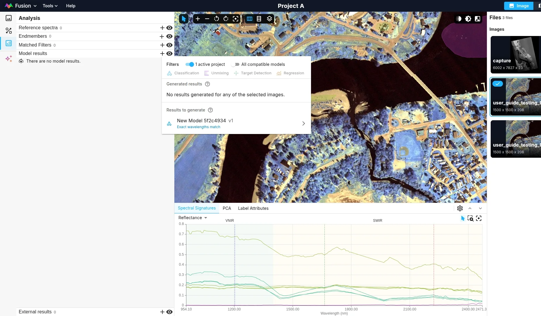
Using the finished model
Once you create a model that meets your performance requirements, you can re-use it on any new image without having to train a new model on that image. Simply upload the image to Clarity Drive, open it in Spectral Explorer, and right click it, selecting "Generate results" to run your image on the model.
Note: Firstly, it is important to ensure that the new image is captured using a similar sensor configuration as the one used to train the model. This includes the spectral bands, center frequencies, and spectral binning options.
Secondly, for the model inference to produce good results, the new images should come from the same distribution as the training images. This means that the spectral signatures in the new images should be similar to the ones used to train
Inference results
You can see inference results either in the results tab of the models page, or in Spectral Explorer.